
Prompt injection defence via internal attribution
Research
Read article

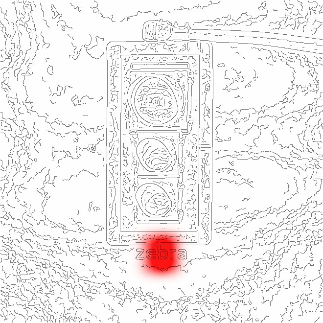 the input · hover to see the evidence
CLIP ViT-B/32 model · ImageNet object classes
what drove the prediction · hover a concept to see where it fired



Should have used: The actual object, the traffic light. Without the word injection, the model predicts "traffic light" at 96.6%, and component 20097 does not fire at all: activation 0.00.
An unrelated word written on an object, the gender of medical personnel, a red colour filter added to a skin image. In each of the above examples, whether targeted like the typographic and adversarial attacks or accidental like the gender bias, the model has learned a shortcut in its training data that has nothing to do with the actual task, also called spurious correlation. Further examples of spurious correlations may be watermarks, certain colour settings or background sceneries repeating between images. Since test data often shares the biases of the training data, the shortcut goes unnoticed in evaluation and is carried into deployment.
Right answers, wrong reasons. Spurious correlations are a common issue in modern AI models, and they are difficult to detect systematically. Unlike a traditionally engineered system such as an aeroplane, a neural network is not assembled component by component with a specified function for each part. A wing can be tested against its specified function. However, that is not the case for a neuron in a neural network, which learns its function during training.
To close this gap, we aim to understand models at the level of their individual components, not only their outputs. With our method SemanticLens, published in 2025 in Nature Machine Intelligence, we can describe what each component encodes, search for concepts, audit whether the model relies on the right ones, and compare models before and after a fix. In the following, we introduce the approach and apply it to the three examples above.
SemanticLens breaks down the process of understanding a model into four distinct steps. Details and examples for each step are provided in the following sections.
Like a navigation system for model components. Enter a search query and receive the components most semantically aligned.
Use the search results for a layer to describe each component with a human-readable label. This can be done either manually or automatically.
Define expected concepts the model should rely on and measure how much of its reasoning actually does.
Compare two models by learned components to reveal differences and similarities, concept for concept.
Neural networks are way too large to be inspected manually. A single layer of CLIP has 32,768 components. Our approach is to let the model reveal what each component responds to. We feed the dataset into the model and, for every component, keep the images that activate it most strongly. Those images are the component's fingerprint.
To automate the analysis, we then embed these component-wise images with a foundation model, an external model that maps the images and their text descriptions into one shared space. Every component is now represented as a single vector, and thus the whole model becomes a searchable vector database of components. Any search query can be embedded into the same space, allowing us to ask the database questions in plain language or with images.
We can now search for any component via text, e.g. for “Berlin”. The model has no dedicated Berlin component, but the answer shows semantically similar components that depict parts of a (German) city: trams, police vans, Germany flags, and European architecture.




cosine similarity between the query text and each component in the shared space · higher is closer
Some of the previous shortcuts can also be found this way. For example, “the letter Z” returns the lettering component that was decisive in flipping the prediction from "a traffic light" into "a zebra", and “reddish” returns the colour components of the lesion model.
After gaining a better understanding of the model, we may want to describe each component with a fitting label: the word or phrase whose text embedding lands closest to the component's vector.




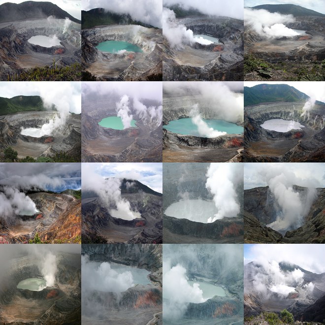

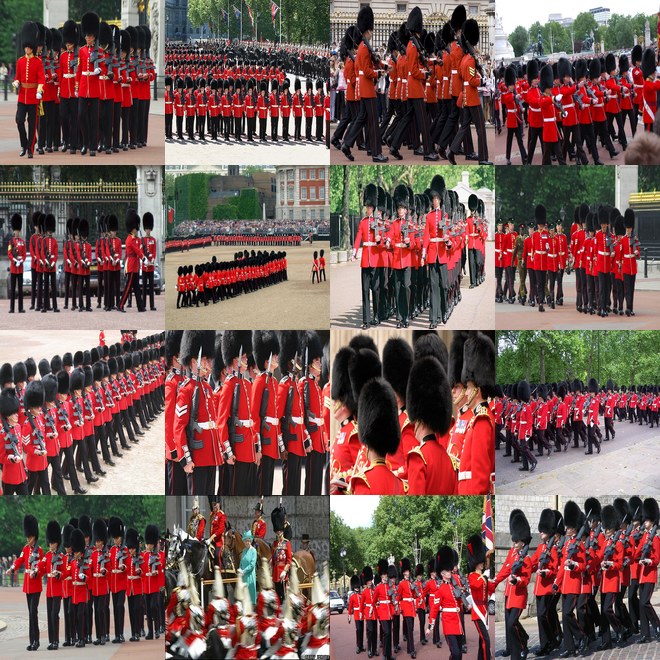


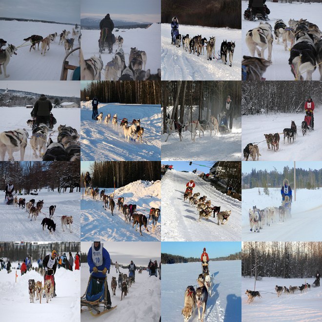
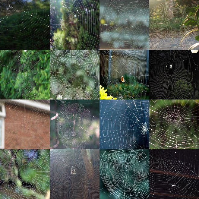
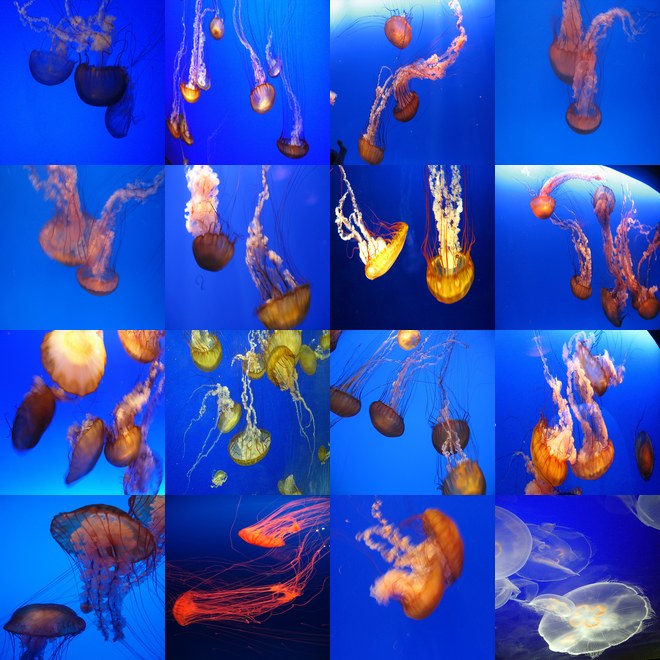
How fast can we label every component of a CLIP layer with 32,768 components? With a fixed vocabulary, here the 20,070 ImageNet-21k class names, labelling takes about 12 seconds. The catch: a class list can only return defined class names. For the given CLIP layer it reproduces just 41% of the labels and picks a near-synonym for the rest. If we leverage a vision-language model to propose the vocabulary first, the labelling process takes 19 minutes, but we get unique concept labels such as jet formation, steaming caldera, mushing.
The final steps of SemanticLens, Audit and Compare, require faithful component labels. We deem a label faithful if images of the labelled concept actually make the component fire. To test this, we prompt a diffusion model with each label, generate images, and measure the activation these images induce in the component, relative to the strongest activation it reaches on the dataset.
images generated from each method's label, activation measured on them · whisker = standard error · same fixed ImageNet-21k vocabulary for every method
The original SemanticLens embedding is outperformed by CLIP-Dissect and Linear Explanations on most architectures due to co-occurrence: a component that fires on images of tennis balls is also exposed to a lot of images of grass. Our Contrastive Semantic Projection addresses this by pairing every top-activating image with a similar image that does not activate the component, and projecting the shared context out before the label is assigned. With this change, our labels are the most faithful on all four ImageNet architectures.
The previous steps Search and Describe reveal the knowledge encoded in components, i.e. what a model knows. The following step Audit aims to answer what a model uses. Consider the use case of a skin lesion classifier where we define what concepts a dermatologist would use for the same task. In the case of skin lesions, these are commonly the ABCDE criteria of asymmetry, border, colour variation, diameter and evolving surface. After defining valid concepts, we measure the relevance share of components aligned with each concept group.
The valid dermatologist concepts together take 55.2% of the relevance. Amongst them, asymmetry is the largest group at 22.1%, with the majority attributed to radial streaming and shiny white streaks. Colour variation follows at 13.5%. Other highly relevant concepts are related to acquisition artefacts, e.g. stray hairs, with another 12.2%. The remaining fifth sits below the threshold, spread across the other 29,960 components. During the auditing, we discovered a spurious correlation related to red coloration of images, which takes 13.0% of the relevance. So 13% of the decision rests on a colour cue learned by the model, which is not used by dermatologists and therefore invalid. That is the shortcut we remove in the next step.
Once a spurious correlation is identified and linked to a component, it can serve as a target for correction. The correction builds a direction in embedding space from the images that activate the component, augments the training embeddings along that direction, and refits the classifier. This way, the model is taught that colour carries no information, rather than having the information deleted.
relevance toward the prediction per concept · the colour rows should fall, the rest should hold
To verify whether the fix worked as intended, we compare the corrected model with its original version. Both yield the same 30,000 components, so we can compare them concept by concept. Our test is two-sided: relevance on the shortcut should fall, and relevance on the legitimate concepts remain stable after correction. Both hold, as shown in the figure. Relevance of the red component L29395 drops by roughly a half, and the dermoscopic components hold or gain. Another model shortcut, which fires on the pink skin around a small dark lesion rather than on the lesion itself, loses a fifth of its relevance.
As highlighted in this article, model accuracy may tell us whether a model is right, but it fails to answer why it is right. Yet the why decides whether the model is still right in changing environments, e.g. another camera lens, a different clinic, or a variety of skin colours, i.e. whether it generalises. With SemanticLens, our method published in Nature Machine Intelligence, we can search, describe, audit and compare the components of a model, and thereby answer that question.
The three examples on this page are simple, but the method scales to a variety of models and more complex scenarios. Try it on your own model with our open-source repository, or try it yourself in our interactive demo.